Example for CESM1

Reference:

- GitHub: https://github.com/ncar/cesm-lens-aws/

- Data/Variables Information: https://ncar.github.io/cesm-lens-aws/#data-catalog

- Reproduce CESM-LENS: http://gallery.pangeo.io/repos/NCAR/cesm-lens-aws/notebooks/kay-et-al-2015.v3.html

Step 0: load necessary packages and define parameters (no need to change)

%%time
# Display output of plots directly in Notebook
%matplotlib inline
import matplotlib.pyplot as plt
import pandas as pd
import json
from flaml import AutoML
from sklearn.metrics import mean_squared_error, r2_score
import warnings
warnings.filterwarnings("ignore")
import util

with open("./config_cesm1.json",'r') as load_f:
#     param = json.loads(json.load(load_f))
    param = json.load(load_f)

    model = param["model"] # cesm1
    city_loc = param["city_loc"] # {"lat": 40.0150, "lon": -105.2705}
    l_component = param["l_component"]
    a_component = param["a_component"]
    experiment = param["experiment"]
    frequency = param["frequency"]
    cam_ls = param["cam_ls"]
    clm_ls = param["clm_ls"]
    time = slice(param["time_start"],param["time_end"])
    member_id = param["member_id"]
    estimator_list = param["estimator_list"]
    time_budget = param["time_budget"]
    features = param["features"]
    label = param["label"]
    clm_var_mask = param["label"][0]

# get a dataset
ds = util.get_data(model, city_loc, experiment, frequency, member_id, time, cam_ls, clm_ls)

# create a dataframe
ds['time'] = ds.indexes['time'].to_datetimeindex()
df = ds.to_dataframe().reset_index().dropna()

if "PRSN" in features:
    df["PRSN"] = df["PRECSC"] + df["PRECSL"]

# setup for automl
automl = AutoML()
automl_settings = {
    "time_budget": time_budget,  # in seconds
    "metric": 'r2',
    "task": 'regression',
    "estimator_list":estimator_list,
}

/glade/work/zhonghua/miniconda3/envs/aws_urban/lib/python3.8/site-packages/xgboost/compat.py:31: FutureWarning: pandas.Int64Index is deprecated and will be removed from pandas in a future version. Use pandas.Index with the appropriate dtype instead.
  from pandas import MultiIndex, Int64Index

--> The keys in the returned dictionary of datasets are constructed as follows:
        'component.experiment.frequency'

100.00% [2/2 00:01<00:00]

CPU times: user 51.6 s, sys: 35.5 s, total: 1min 27s
Wall time: 59.9 s

Step 1: data analysis

xarray.Dataset

ds

<xarray.Dataset>
Dimensions:     (member_id: 1, time: 7299)
Coordinates:
  * member_id   (member_id) int64 2
    lat         float64 40.05
    lon         float64 255.0
  * time        (time) datetime64[ns] 2081-01-02T12:00:00 ... 2100-12-31T12:0...
Data variables:
    TREFHT      (member_id, time) float32 255.8 266.8 271.1 ... 277.6 276.1
    TREFHTMX    (member_id, time) float32 269.3 278.4 281.2 ... 283.9 277.5
    FLNS        (member_id, time) float32 77.09 67.4 77.49 ... 64.89 37.45 38.35
    FSNS        (member_id, time) float32 83.31 88.83 90.25 ... 67.98 80.27
    PRECSC      (member_id, time) float32 0.0 0.0 0.0 0.0 ... 0.0 0.0 8.927e-12
    PRECSL      (member_id, time) float32 4.887e-10 6.665e-10 ... 9.722e-10
    PRECT       (member_id, time) float32 4.887e-10 6.665e-10 ... 2.32e-08
    QBOT        (member_id, time) float32 0.000913 0.001889 ... 0.005432 0.00492
    UBOT        (member_id, time) float32 5.461 4.815 4.506 ... 2.865 3.255
    VBOT        (member_id, time) float32 1.27 3.189 3.691 ... 1.215 0.8704
    TREFMXAV_U  (member_id, time) float32 259.6 270.0 279.8 ... 284.9 285.3
Attributes: (12/14)
    intake_esm_varname:        FLNS\nFSNS\nPRECSC\nPRECSL\nPRECT\nQBOT\nTREFH...
    topography_file:           /scratch/p/pjk/mudryk/cesm1_1_2_LENS/inputdata...
    title:                     UNSET
    Version:                   $Name$
    NCO:                       4.4.2
    host:                      tcs-f02n07
    ...                        ...
    important_note:            This data is part of the project 'Blind Evalua...
    initial_file:              b.e11.B20TRC5CNBDRD.f09_g16.105.cam.i.2006-01-...
    source:                    CAM
    revision_Id:               $Id$
    logname:                   mudryk
    intake_esm_dataset_key:    atm.RCP85.daily

xarray.Dataset

• Dimensions:
  • member_id: 1
  • time: 7299
• Coordinates: (4)
  • member_id
    (member_id)
    int64
    2

    array([2])

  • lat
    ()
    float64
    40.05

    axis :

    Y

    bounds :

    lat_bnds

    long_name :

    latitude

    standard_name :

    latitude

    units :

    degrees_north

    array(40.05235672)

  • lon
    ()
    float64
    255.0

    long_name :

    longitude

    units :

    degrees_east

    array(255.)

  • time
    (time)
    datetime64[ns]
    2081-01-02T12:00:00 ... 2100-12-...

    array(['2081-01-02T12:00:00.000000000', '2081-01-03T12:00:00.000000000',
           '2081-01-04T12:00:00.000000000', ..., '2100-12-29T12:00:00.000000000',
           '2100-12-30T12:00:00.000000000', '2100-12-31T12:00:00.000000000'],
          dtype='datetime64[ns]')

• Data variables: (11)
  • TREFHT
    (member_id, time)
    float32
    255.8 266.8 271.1 ... 277.6 276.1

    cell_methods :

    time: mean

    long_name :

    Reference height temperature

    units :

    K

    array([[255.84972, 266.79083, 271.12204, ..., 275.39145, 277.6332 ,
            276.08655]], dtype=float32)

  • TREFHTMX
    (member_id, time)
    float32
    269.3 278.4 281.2 ... 283.9 277.5

    cell_methods :

    time: maximum

    long_name :

    Maximum reference height temperature over output period

    units :

    K

    array([[269.32785, 278.39655, 281.18195, ..., 283.58582, 283.92764,
            277.4649 ]], dtype=float32)

  • FLNS
    (member_id, time)
    float32
    77.09 67.4 77.49 ... 37.45 38.35

    Sampling_Sequence :

    rad_lwsw

    cell_methods :

    time: mean

    long_name :

    Net longwave flux at surface

    units :

    W/m2

    array([[77.0858  , 67.40266 , 77.493195, ..., 64.88807 , 37.445972,
            38.35395 ]], dtype=float32)

  • FSNS
    (member_id, time)
    float32
    83.31 88.83 90.25 ... 67.98 80.27

    Sampling_Sequence :

    rad_lwsw

    cell_methods :

    time: mean

    long_name :

    Net solar flux at surface

    units :

    W/m2

    array([[83.311066, 88.83119 , 90.24748 , ..., 87.44088 , 67.978905,
            80.26761 ]], dtype=float32)

  • PRECSC
    (member_id, time)
    float32
    0.0 0.0 0.0 ... 0.0 0.0 8.927e-12

    cell_methods :

    time: mean

    long_name :

    Convective snow rate (water equivalent)

    units :

    m/s

    array([[0.0000000e+00, 0.0000000e+00, 0.0000000e+00, ..., 0.0000000e+00,
            0.0000000e+00, 8.9266485e-12]], dtype=float32)

  • PRECSL
    (member_id, time)
    float32
    4.887e-10 6.665e-10 ... 9.722e-10

    cell_methods :

    time: mean

    long_name :

    Large-scale (stable) snow rate (water equivalent)

    units :

    m/s

    array([[4.8865317e-10, 6.6647016e-10, 8.0305154e-14, ..., 4.6877151e-23,
            6.2482954e-19, 9.7219222e-10]], dtype=float32)

  • PRECT
    (member_id, time)
    float32
    4.887e-10 6.665e-10 ... 2.32e-08

    cell_methods :

    time: mean

    long_name :

    Total (convective and large-scale) precipitation rate (liq + ice)

    units :

    m/s

    array([[4.8865317e-10, 6.6652112e-10, 2.5380477e-11, ..., 7.4445916e-10,
            6.5936290e-10, 2.3197726e-08]], dtype=float32)

  • QBOT
    (member_id, time)
    float32
    0.000913 0.001889 ... 0.00492

    cell_methods :

    time: mean

    long_name :

    Lowest model level water vapor mixing ratio

    units :

    kg/kg

    array([[0.00091295, 0.00188927, 0.00333069, ..., 0.00430955, 0.00543191,
            0.00492025]], dtype=float32)

  • UBOT
    (member_id, time)
    float32
    5.461 4.815 4.506 ... 2.865 3.255

    cell_methods :

    time: mean

    long_name :

    Lowest model level zonal wind

    units :

    m/s

    array([[5.461293 , 4.814545 , 4.5064588, ..., 5.497996 , 2.8646276,
            3.254671 ]], dtype=float32)

  • VBOT
    (member_id, time)
    float32
    1.27 3.189 3.691 ... 1.215 0.8704

    cell_methods :

    time: mean

    long_name :

    Lowest model level meridional wind

    units :

    m/s

    array([[1.2702359 , 3.1894999 , 3.6906984 , ..., 1.3250201 , 1.2154012 ,
            0.87040335]], dtype=float32)

  • TREFMXAV_U
    (member_id, time)
    float32
    259.6 270.0 279.8 ... 284.9 285.3

    cell_methods :

    time: mean

    long_name :

    Urban daily maximum of average 2-m temperature

    units :

    K

    array([[259.64197, 269.9728 , 279.82883, ..., 283.00278, 284.9374 ,
            285.26486]], dtype=float32)

• Attributes: (14)

  intake_esm_varname :

  FLNS FSNS PRECSC PRECSL PRECT QBOT TREFHT TREFHTMX UBOT VBOT

  topography_file :

  /scratch/p/pjk/mudryk/cesm1_1_2_LENS/inputdata/atm/cam/topo/USGS-gtopo30_0.9x1.25_remap_c051027.nc

  title :

  UNSET

  Version :

  $Name$

  NCO :

  4.4.2

  host :

  tcs-f02n07

  nco_openmp_thread_number :

  1

  Conventions :

  CF-1.0

  important_note :

  This data is part of the project 'Blind Evaluation of Lossy Data-Compression in LENS'. Please exercise caution before using this data for other purposes.

  initial_file :

  b.e11.B20TRC5CNBDRD.f09_g16.105.cam.i.2006-01-01-00000.nc

  source :

  CAM

  revision_Id :

  $Id$

  logname :

  mudryk

  intake_esm_dataset_key :

  atm.RCP85.daily

pandas dataframe

df.head()

	member_id	time	TREFHT	TREFHTMX	FLNS	FSNS	PRECSC	PRECSL	PRECT	QBOT	UBOT	VBOT	lat	lon	TREFMXAV_U	PRSN
0	2	2081-01-02 12:00:00	255.849716	269.327850	77.085800	83.311066	0.0	4.886532e-10	4.886532e-10	0.000913	5.461293	1.270236	40.052357	255.0	259.641968	4.886532e-10
1	2	2081-01-03 12:00:00	266.790833	278.396545	67.402657	88.831192	0.0	6.664702e-10	6.665211e-10	0.001889	4.814545	3.189500	40.052357	255.0	269.972809	6.664702e-10
2	2	2081-01-04 12:00:00	271.122040	281.181946	77.493195	90.247482	0.0	8.030515e-14	2.538048e-11	0.003331	4.506459	3.690698	40.052357	255.0	279.828827	8.030515e-14
3	2	2081-01-05 12:00:00	276.329895	281.844543	64.789749	93.343193	0.0	1.896001e-20	2.508245e-09	0.004209	5.162941	4.963157	40.052357	255.0	282.674103	1.896001e-20
4	2	2081-01-06 12:00:00	275.347229	280.980469	69.647041	80.993706	0.0	5.442079e-17	7.844814e-09	0.004014	4.478484	4.272586	40.052357	255.0	283.518707	5.442079e-17

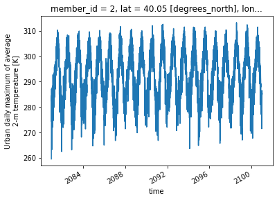
data visualization

ds["TREFMXAV_U"].plot()

[<matplotlib.lines.Line2D at 0x2b3bfa600a00>]

Step 2: automated machine learning

train a model (emulator)

%%time
# assume that we want to split the data into training data and testing data
# let's use first 95% for training, and the remaining for testing
idx = df.shape[0]
train = df.iloc[:int(0.95*idx),:]
test = df.iloc[int(0.95*idx):,:]
(X_train, y_train) = (train[features], train[label].values)
(X_test, y_test) = (test[features], test[label].values)

# train the model
automl.fit(X_train=X_train, y_train=y_train,
           **automl_settings, verbose=-1)
print(automl.model.estimator)

XGBRegressor(base_score=0.5, booster='gbtree',
             colsample_bylevel=0.8981353296453468, colsample_bynode=1,
             colsample_bytree=0.8589079860800738, gamma=0, gpu_id=-1,
             grow_policy='lossguide', importance_type='gain',
             interaction_constraints='', learning_rate=0.05211228610238813,
             max_delta_step=0, max_depth=0, max_leaves=29,
             min_child_weight=45.3846760978798, missing=nan,
             monotone_constraints='()', n_estimators=299, n_jobs=-1,
             num_parallel_tree=1, random_state=0, reg_alpha=0.01917865165509354,
             reg_lambda=2.2296607355174927, scale_pos_weight=1,
             subsample=0.9982731696185565, tree_method='hist',
             use_label_encoder=False, validate_parameters=1, verbosity=0)
CPU times: user 3min 35s, sys: 2.67 s, total: 3min 38s
Wall time: 15.7 s

apply and test the machine learning model

use automl.predict(X) to apply the model

# training data
print("model performance using training data:")
y_pred = automl.predict(X_train)
print("root mean square error:",
      mean_squared_error(y_true=y_train, y_pred=y_pred, squared=False))
print("r2:", r2_score(y_true=y_train, y_pred=y_pred),"\n")
import pandas as pd
d_train = {"time":train["time"],"y_train":y_train.reshape(-1),"y_pred":y_pred.reshape(-1)}
df_train = pd.DataFrame(d_train).set_index("time")

# testing data
print("model performance using testing data:")
y_pred = automl.predict(X_test)
print("root mean square error:",
      mean_squared_error(y_true=y_test, y_pred=y_pred, squared=False))
print("r2:", r2_score(y_true=y_test, y_pred=y_pred))
d_test = {"time":test["time"],"y_test":y_test.reshape(-1),"y_pred":y_pred.reshape(-1)}
df_test = pd.DataFrame(d_test).set_index("time")

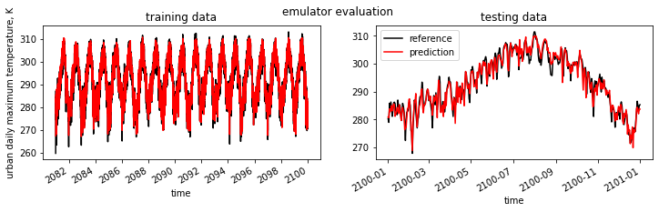
model performance using training data:
root mean square error: 1.7566193
r2: 0.9681344385429989

model performance using testing data:
root mean square error: 2.3287773
r2: 0.9384653117109892

visualization

fig, (ax1,ax2) = plt.subplots(1,2,figsize=(12,3))
fig.suptitle('emulator evaluation')
df_train["y_train"].plot(label="reference",c="k",ax=ax1)
df_train["y_pred"].plot(label="prediction",c="r",ax=ax1)
ax1.set_title("training data")
ax1.set_ylabel("urban daily maximum temperature, K")

df_test["y_test"].plot(label="reference",c="k",ax=ax2)
df_test["y_pred"].plot(label="prediction",c="r",ax=ax2)
ax2.set_title("testing data")
plt.legend()
plt.show()