Example for CMIP6
Here, CESM2 data serves as the training data, and the ML model trained on CESM2 data is applied to CMIP6 data.
Reference:
- GitHub: https://github.com/NCAR/cesm2-le-aws
- Data/Variables Information: - https://ncar.github.io/cesm2-le-aws/model_documentation.html#data-catalog
- Reproduce CESM-LENS: https://github.com/NCAR/cesm2-le-aws/blob/main/notebooks/kay_et_al_lens2.ipynb
Step 0: load necessary packages and define parameters (no need to change)
[1]:
%%time
# Display output of plots directly in Notebook
%matplotlib inline
import matplotlib.pyplot as plt
import pandas as pd
import json
import intake
from flaml import AutoML
from sklearn.metrics import mean_squared_error, r2_score
from sklearn.model_selection import train_test_split
import warnings
warnings.filterwarnings("ignore")
import util
import math
import seaborn as sns

with open("./config_cesm2_cmip6.json",'r') as load_f:
#     param = json.loads(json.load(load_f))
    param = json.load(load_f)

    model = param["model"] # cesm2
    urban_type = param["urban_type"] # md
    city_loc = param["city_loc"] # {"lat": 40.0150, "lon": -105.2705}
    l_component = param["l_component"]
    a_component = param["a_component"]
    experiment = param["experiment"]
    frequency = param["frequency"]
    cam_ls = param["cam_ls"]
    clm_ls = param["clm_ls"]
    forcing_variant = param["forcing_variant"]
    time = slice(param["time_start"],param["time_end"])
    member_id = param["member_id"]
    estimator_list = param["estimator_list"]
    time_budget = param["time_budget"]
    features = param["features"]
    label = param["label"]
    clm_var_mask = param["label"][0]
    CMIP6_url = param["CMIP6_url"]
    activity_id = param["activity_id"]
    experiment_id = param["experiment_id"]
    institution_id = param["institution_id"]
    table_id = param["table_id"]
CPU times: user 1.84 s, sys: 350 ms, total: 2.19 s
Wall time: 2.19 s
/glade/work/zhonghua/miniconda3/envs/aws_urban/lib/python3.8/site-packages/xgboost/compat.py:31: FutureWarning: pandas.Int64Index is deprecated and will be removed from pandas in a future version. Use pandas.Index with the appropriate dtype instead.
  from pandas import MultiIndex, Int64Index
Step 1: load CESM2 data
[2]:
# get a dataset
ds = util.get_data(model, city_loc, experiment, frequency, member_id, time, cam_ls, clm_ls,
                   forcing_variant=forcing_variant, urban_type=urban_type)
ds['time'] = ds.indexes['time'].to_datetimeindex()
--> The keys in the returned dictionary of datasets are constructed as follows:
        'component.experiment.frequency.forcing_variant'
100.00% [2/2 00:01<00:00]
different lat between CAM and CLM subgrid info, adjust subgrid info's lat
split into training and testing data
[3]:
mapping =  {
    "PRSN":"prsn",
    "PRECT":"pr",
    "PSL":"psl",
    "TREFHT":"tas",
    "TREFHTMN":"tasmin",
    "TREFHTMX":"tasmax"
}

# create a dataframe
df = ds.to_dataframe().reset_index().dropna()
df["PRSN"] = (df["PRECSC"] + df["PRECSL"])*1000
df["PRECT"] = (df["PRECC"] + df["PRECL"])*1000

df_cesm = df.rename(columns=mapping)

# split the data into training and testing data
X_train, X_test, y_train, y_test = train_test_split(
    df_cesm[features], df_cesm[label], test_size=0.1, random_state=42)
display(X_train.head())
display(y_train.head())
| pr | prsn | psl | tas | tasmax | tasmin | |
|---|---|---|---|---|---|---|
| 4253 | 5.120080e-05 | 1.210190e-18 | 102141.148438 | 297.131683 | 305.057770 | 291.910309 |
| 712 | 8.689989e-06 | 4.476514e-06 | 102655.820312 | 273.535492 | 277.919128 | 270.931824 |
| 4174 | 5.766846e-05 | 2.315565e-14 | 101171.445312 | 297.524048 | 305.175293 | 290.375336 |
| 1811 | 8.906457e-07 | 7.931703e-07 | 101316.953125 | 271.924591 | 277.630005 | 269.025482 |
| 5097 | 4.478946e-08 | 4.477884e-08 | 101735.164062 | 270.995270 | 275.632812 | 269.006317 |
| TREFMXAV | |
|---|---|
| 4253 | 305.300262 |
| 712 | 279.708527 |
| 4174 | 306.675201 |
| 1811 | 278.521729 |
| 5097 | 276.521973 |
Step 2: load CMIP6 data
[4]:
%%time
features = ['pr', 'prsn', 'psl','tas', 'tasmax', 'tasmin']

catalog = intake.open_esm_datastore('https://cmip6-pds.s3.amazonaws.com/pangeo-cmip6.json')
catalog_subset = catalog.search(
    activity_id=activity_id,
    experiment_id=experiment_id,
    institution_id=institution_id,
    variable_id=features,
    table_id=table_id
)
datasets = catalog_subset.to_dataset_dict(zarr_kwargs={'consolidated': True, 'decode_times': True})
datasets
--> The keys in the returned dictionary of datasets are constructed as follows:
        'activity_id.institution_id.source_id.experiment_id.table_id.grid_label'
100.00% [1/1 00:00<00:00]
CPU times: user 8.71 s, sys: 973 ms, total: 9.69 s
Wall time: 17 s
[4]:
{'ScenarioMIP.NOAA-GFDL.GFDL-ESM4.ssp370.day.gr1': <xarray.Dataset>
 Dimensions:    (bnds: 2, lat: 180, lon: 288, member_id: 1, time: 31390)
 Coordinates:
   * bnds       (bnds) float64 1.0 2.0
   * lat        (lat) float64 -89.5 -88.5 -87.5 -86.5 ... 86.5 87.5 88.5 89.5
     lat_bnds   (lat, bnds) float64 dask.array<chunksize=(180, 2), meta=np.ndarray>
   * lon        (lon) float64 0.625 1.875 3.125 4.375 ... 355.6 356.9 358.1 359.4
     lon_bnds   (lon, bnds) float64 dask.array<chunksize=(288, 2), meta=np.ndarray>
   * time       (time) object 2015-01-01 12:00:00 ... 2100-12-31 12:00:00
     time_bnds  (time, bnds) object dask.array<chunksize=(15695, 2), meta=np.ndarray>
   * member_id  (member_id) <U8 'r1i1p1f1'
     height     float64 2.0
 Data variables:
     pr         (member_id, time, lat, lon) float32 dask.array<chunksize=(1, 592, 180, 288), meta=np.ndarray>
     prsn       (member_id, time, lat, lon) float32 dask.array<chunksize=(1, 671, 180, 288), meta=np.ndarray>
     psl        (member_id, time, lat, lon) float32 dask.array<chunksize=(1, 452, 180, 288), meta=np.ndarray>
     tas        (member_id, time, lat, lon) float32 dask.array<chunksize=(1, 420, 180, 288), meta=np.ndarray>
     tasmax     (member_id, time, lat, lon) float32 dask.array<chunksize=(1, 420, 180, 288), meta=np.ndarray>
     tasmin     (member_id, time, lat, lon) float32 dask.array<chunksize=(1, 415, 180, 288), meta=np.ndarray>
 Attributes: (12/48)
     references:              see further_info_url attribute
     realm:                   atmos
     parent_time_units:       days since 1850-1-1
     sub_experiment:          none
     forcing_index:           1
     grid_label:              gr1
     ...                      ...
     parent_variant_label:    r1i1p1f1
     license:                 CMIP6 model data produced by NOAA-GFDL is licens...
     parent_mip_era:          CMIP6
     parent_activity_id:      CMIP
     title:                   NOAA GFDL GFDL-ESM4 model output prepared for CM...
     intake_esm_dataset_key:  ScenarioMIP.NOAA-GFDL.GFDL-ESM4.ssp370.day.gr1}
[5]:
%%time
# define the dataset name in the dictionary and the "member_id"
df_cmip = datasets['ScenarioMIP.NOAA-GFDL.GFDL-ESM4.ssp370.day.gr1']\
          .sel(member_id = 'r1i1p1f1',
               time = slice(param["time_start"], param["time_end"]))\
          .sel(lat = param["city_loc"]["lat"],
               lon = util.lon_to_360(param["city_loc"]["lon"]),
               method="nearest")\
          [features].load()\
          .to_dataframe().reset_index()
df_cmip.head()
CPU times: user 20.3 s, sys: 11 s, total: 31.3 s
Wall time: 18.5 s
[5]:
| time | pr | prsn | psl | tas | tasmax | tasmin | lat | lon | member_id | height | |
|---|---|---|---|---|---|---|---|---|---|---|---|
| 0 | 2081-01-02 12:00:00 | 4.284881e-11 | 1.210498e-13 | 101005.351562 | 267.040985 | 274.020386 | 264.221344 | 40.5 | 254.375 | r1i1p1f1 | 2.0 |
| 1 | 2081-01-03 12:00:00 | 1.998000e-06 | 6.424573e-07 | 100812.898438 | 272.238739 | 275.491943 | 270.209229 | 40.5 | 254.375 | r1i1p1f1 | 2.0 |
| 2 | 2081-01-04 12:00:00 | 1.482927e-05 | 8.858435e-06 | 100455.796875 | 273.498535 | 274.920624 | 271.907166 | 40.5 | 254.375 | r1i1p1f1 | 2.0 |
| 3 | 2081-01-05 12:00:00 | 6.613790e-06 | 5.915619e-06 | 101060.375000 | 271.265442 | 273.210297 | 269.065277 | 40.5 | 254.375 | r1i1p1f1 | 2.0 |
| 4 | 2081-01-06 12:00:00 | 9.097347e-06 | 6.341099e-06 | 100795.867188 | 272.010651 | 276.695343 | 269.123260 | 40.5 | 254.375 | r1i1p1f1 | 2.0 |
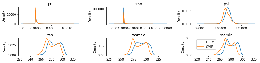
Step 3: compare CESM2 training and CMIP6 data
[6]:
fig = plt.figure(figsize=(12,3))
idx = 1
for var in features:
    ax = fig.add_subplot(math.ceil(math.ceil(len(features)/3)), 3, idx)
    X_train[var].plot.kde(ax=ax, label="CESM")
    df_cmip[var].plot.kde(ax=ax, label="CMIP")
    idx+=1
    ax.set_title(var)
plt.legend()
plt.tight_layout()
plt.show()
Step 4: automated machine learning
train a model (emulator)
[7]:
%%time
# setup for automl
automl = AutoML()
automl_settings = {
    "time_budget": time_budget,  # in seconds
    "metric": 'r2',
    "task": 'regression',
    "estimator_list":estimator_list,
}

# train the model
automl.fit(X_train=X_train, y_train=y_train.values,
           **automl_settings, verbose=-1)
print(automl.model.estimator)
ExtraTreesRegressor(max_features=0.9591245274694429, max_leaf_nodes=426,
                    n_estimators=125, n_jobs=-1)
CPU times: user 2min 1s, sys: 2.9 s, total: 2min 4s
Wall time: 15.2 s
evaluate the model
[8]:
y_pred = automl.predict(X_test)
print("root mean square error:",
      round(mean_squared_error(y_true=y_test, y_pred=y_pred, squared=False),3))
print("r2:",
      round(r2_score(y_true=y_test, y_pred=y_pred),3))
root mean square error: 0.636
r2: 0.997
apply and test the machine learning model
use
automl.predict(X) to apply the model[9]:
df_cmip[label] = automl.predict(df_cmip[features]).reshape(df_cmip.shape[0],-1)
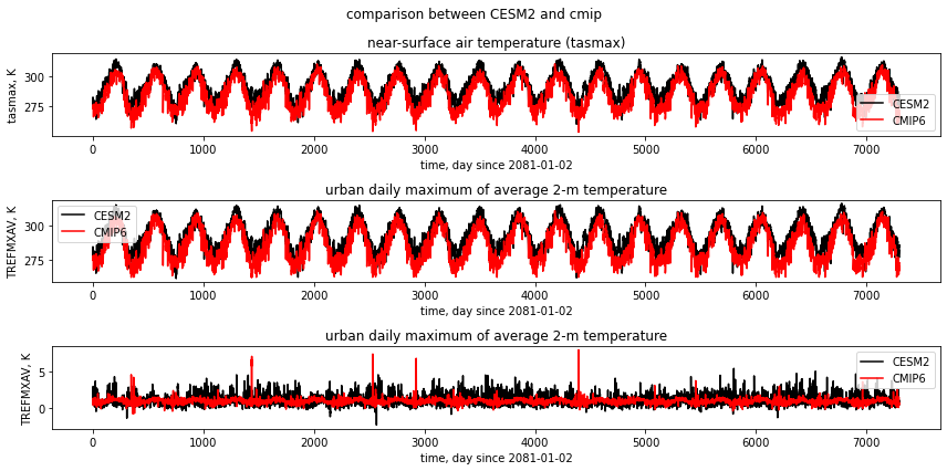
Step 5: visualization
[10]:
fig, (ax1,ax2,ax3) = plt.subplots(3,1,figsize=(12,6))
fig.suptitle('comparison between CESM2 and cmip')
df_cesm["tasmax"].plot(label="CESM2",c="k",ax=ax1)
df_cmip["tasmax"].plot(label="cmip",c="r",ax=ax1)
ax1.set_title("near-surface air temperature (tasmax)")
ax1.set_ylabel("tasmax, K")
ax1.set_xlabel("time, day since 2081-01-02")
ax1.legend(["CESM2","CMIP6"])

df_cesm["TREFMXAV"].plot(label="CESM2",c="k",ax=ax2)
df_cmip["TREFMXAV"].plot(label="cmip",c="r",ax=ax2)
ax2.set_title("urban daily maximum of average 2-m temperature")
ax2.set_ylabel("TREFMXAV, K")
ax2.set_xlabel("time, day since 2081-01-02")
ax2.legend(["CESM2","CMIP6"])

(df_cesm["TREFMXAV"]-df_cesm["tasmax"]).plot(label="CESM2",c="k",ax=ax3)
(df_cmip["TREFMXAV"]-df_cmip["tasmax"]).plot(label="cmip",c="r",ax=ax3)
ax3.set_title("urban daily maximum of average 2-m temperature")
ax3.set_ylabel("TREFMXAV, K")
ax3.set_xlabel("time, day since 2081-01-02")
ax3.legend(["CESM2","CMIP6"])

plt.tight_layout()
plt.show()
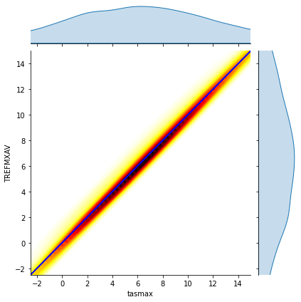
[11]:
# reference: https://stackoverflow.com/questions/53964485/seaborn-jointplot-color-by-density
x = df_cesm["tasmax"]-df_cmip["tasmax"]
y = df_cesm["TREFMXAV"]-df_cmip["TREFMXAV"]

plot = sns.jointplot(x, y, kind="kde", cmap='hot_r', n_levels=60, fill=True)
plot.ax_joint.set_xlim(-2.5,15)
plot.ax_joint.set_ylim(-2.5,15)
plot.ax_joint.plot([-2.5,15], [-2.5,15], 'b-', linewidth = 2)
plt.show()
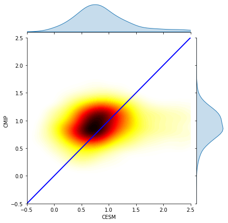
[12]:
# reference: https://stackoverflow.com/questions/53964485/seaborn-jointplot-color-by-density
x = df_cesm["TREFMXAV"]-df_cesm["tasmax"]
y = df_cmip["TREFMXAV"]-df_cmip["tasmax"]

plot = sns.jointplot(x, y, kind="kde", cmap='hot_r', n_levels=60, fill=True)
plot.ax_joint.set_xlim(-0.5,2.5)
plot.ax_joint.set_ylim(-0.5,2.5)
plot.ax_joint.set_xlabel("CESM")
plot.ax_joint.set_ylabel("CMIP")
plot.ax_joint.plot([-0.5,2.5], [-0.5,2.5], 'b-', linewidth = 2)
plt.show()