Example for CESM2

NOTE: Compared to the CESM1 demo, here “Q” (QBOT), “U” (UBOT) and “V” (VBOT) are not included. When the bottom “lev” of “Q”, “U”, and “V” are merged, there is an issue.

Reference:

- GitHub: https://github.com/NCAR/cesm2-le-aws

- Data/Variables Information: https://ncar.github.io/cesm2-le-aws/model_documentation.html#data-catalog

- Reproduce CESM-LENS: https://github.com/NCAR/cesm2-le-aws/blob/main/notebooks/kay_et_al_lens2.ipynb

Step 0: load necessary packages and define parameters (no need to change)

%%time
# Display output of plots directly in Notebook
%matplotlib inline
import matplotlib.pyplot as plt
import pandas as pd
import json
from flaml import AutoML
from sklearn.metrics import mean_squared_error, r2_score
import warnings
warnings.filterwarnings("ignore")
import util

with open("./config_cesm2.json",'r') as load_f:
#     param = json.loads(json.load(load_f))
    param = json.load(load_f)

    model = param["model"] # cesm2
    urban_type = param["urban_type"] # md
    city_loc = param["city_loc"] # {"lat": 40.0150, "lon": -105.2705}
    l_component = param["l_component"]
    a_component = param["a_component"]
    experiment = param["experiment"]
    frequency = param["frequency"]
    cam_ls = param["cam_ls"]
    clm_ls = param["clm_ls"]
    forcing_variant = param["forcing_variant"]
    time = slice(param["time_start"],param["time_end"])
    member_id = param["member_id"]
    estimator_list = param["estimator_list"]
    time_budget = param["time_budget"]
    features = param["features"]
    label = param["label"]
    clm_var_mask = param["label"][0]

# get a dataset
ds = util.get_data(model, city_loc, experiment, frequency, member_id, time, cam_ls, clm_ls,
                   forcing_variant=forcing_variant, urban_type=urban_type)

# create a dataframe
ds['time'] = ds.indexes['time'].to_datetimeindex()
df = ds.to_dataframe().reset_index().dropna()

if "PRSN" in features:
    df["PRSN"] = df["PRECSC"] + df["PRECSL"]
if "PRECT" in features:
    df["PRECT"] = df["PRECC"] + df["PRECL"]

# setup for automl
automl = AutoML()
automl_settings = {
    "time_budget": time_budget,  # in seconds
    "metric": 'r2',
    "task": 'regression',
    "estimator_list":estimator_list,
}

/glade/work/zhonghua/miniconda3/envs/aws_urban/lib/python3.8/site-packages/xgboost/compat.py:31: FutureWarning: pandas.Int64Index is deprecated and will be removed from pandas in a future version. Use pandas.Index with the appropriate dtype instead.
  from pandas import MultiIndex, Int64Index

--> The keys in the returned dictionary of datasets are constructed as follows:
        'component.experiment.frequency.forcing_variant'

100.00% [2/2 00:01<00:00]

different lat between CAM and CLM subgrid info, adjust subgrid info's lat
CPU times: user 56.9 s, sys: 34 s, total: 1min 30s
Wall time: 58.4 s

Step 1: data analysis

xarray.Dataset

ds

<xarray.Dataset>
Dimensions:    (member_id: 1, time: 7299)
Coordinates:
    lat        float64 40.05
    lon        float64 255.0
  * member_id  (member_id) <U12 'r1i1231p1f1'
  * time       (time) datetime64[ns] 2081-01-02T12:00:00 ... 2100-12-31T12:00:00
Data variables:
    TREFHT     (member_id, time) float32 273.2 273.4 275.7 ... 276.7 277.0 277.4
    TREFHTMX   (member_id, time) float32 276.2 278.8 282.8 ... 283.9 284.8 283.7
    FLNS       (member_id, time) float32 93.1 82.03 82.87 ... 88.49 87.6 67.41
    FSNS       (member_id, time) float32 90.73 84.27 91.37 ... 91.55 91.45 77.9
    PRECSC     (member_id, time) float32 0.0 0.0 0.0 0.0 0.0 ... 0.0 0.0 0.0 0.0
    PRECSL     (member_id, time) float32 4.184e-10 4.287e-10 ... 9.825e-21
    PRECC      (member_id, time) float32 0.0 0.0 0.0 0.0 0.0 ... 0.0 0.0 0.0 0.0
    PRECL      (member_id, time) float32 4.251e-10 4.42e-10 ... 1.181e-08
    TREFMXAV   (member_id, time) float64 277.0 279.3 284.4 ... 284.3 285.7 284.4
Attributes:
    host:                    mom1
    topography_file:         /mnt/lustre/share/CESM/cesm_input/atm/cam/topo/f...
    logname:                 sunseon
    time_period_freq:        day_1
    intake_esm_varname:      FLNS\nFSNS\nPRECC\nPRECL\nPRECSC\nPRECSL\nTREFHT...
    Conventions:             CF-1.0
    model_doi_url:           https://doi.org/10.5065/D67H1H0V
    source:                  CAM
    intake_esm_dataset_key:  atm.ssp370.daily.cmip6

xarray.Dataset

• Dimensions:
  • member_id: 1
  • time: 7299
• Coordinates: (4)
  • lat
    ()
    float64
    40.05

    long_name :

    latitude

    units :

    degrees_north

    array(40.05235602)

  • lon
    ()
    float64
    255.0

    long_name :

    longitude

    units :

    degrees_east

    array(255.)

  • member_id
    (member_id)
    <U12
    'r1i1231p1f1'

    array(['r1i1231p1f1'], dtype='<U12')

  • time
    (time)
    datetime64[ns]
    2081-01-02T12:00:00 ... 2100-12-...

    array(['2081-01-02T12:00:00.000000000', '2081-01-03T12:00:00.000000000',
           '2081-01-04T12:00:00.000000000', ..., '2100-12-29T12:00:00.000000000',
           '2100-12-30T12:00:00.000000000', '2100-12-31T12:00:00.000000000'],
          dtype='datetime64[ns]')

• Data variables: (9)
  • TREFHT
    (member_id, time)
    float32
    273.2 273.4 275.7 ... 277.0 277.4

    cell_methods :

    time: mean

    long_name :

    Reference height temperature

    units :

    K

    array([[273.18002, 273.39667, 275.67584, ..., 276.73038, 277.025  ,
            277.40417]], dtype=float32)

  • TREFHTMX
    (member_id, time)
    float32
    276.2 278.8 282.8 ... 284.8 283.7

    cell_methods :

    time: maximum

    long_name :

    Maximum reference height temperature over output period

    units :

    K

    array([[276.1923 , 278.82355, 282.8261 , ..., 283.89755, 284.8469 ,
            283.73743]], dtype=float32)

  • FLNS
    (member_id, time)
    float32
    93.1 82.03 82.87 ... 87.6 67.41

    Sampling_Sequence :

    rad_lwsw

    cell_methods :

    time: mean

    long_name :

    Net longwave flux at surface

    units :

    W/m2

    array([[93.097984, 82.03214 , 82.87059 , ..., 88.493256, 87.5951  ,
            67.411705]], dtype=float32)

  • FSNS
    (member_id, time)
    float32
    90.73 84.27 91.37 ... 91.45 77.9

    Sampling_Sequence :

    rad_lwsw

    cell_methods :

    time: mean

    long_name :

    Net solar flux at surface

    units :

    W/m2

    array([[90.73479 , 84.271416, 91.365944, ..., 91.54785 , 91.45452 ,
            77.90161 ]], dtype=float32)

  • PRECSC
    (member_id, time)
    float32
    0.0 0.0 0.0 0.0 ... 0.0 0.0 0.0 0.0

    cell_methods :

    time: mean

    long_name :

    Convective snow rate (water equivalent)

    units :

    m/s

    array([[0., 0., 0., ..., 0., 0., 0.]], dtype=float32)

  • PRECSL
    (member_id, time)
    float32
    4.184e-10 4.287e-10 ... 9.825e-21

    cell_methods :

    time: mean

    long_name :

    Large-scale (stable) snow rate (water equivalent)

    units :

    m/s

    array([[4.1836259e-10, 4.2873260e-10, 1.4922830e-15, ..., 2.0208434e-14,
            2.9697208e-21, 9.8254048e-21]], dtype=float32)

  • PRECC
    (member_id, time)
    float32
    0.0 0.0 0.0 0.0 ... 0.0 0.0 0.0 0.0

    cell_methods :

    time: mean

    long_name :

    Convective precipitation rate (liq + ice)

    units :

    m/s

    array([[0., 0., 0., ..., 0., 0., 0.]], dtype=float32)

  • PRECL
    (member_id, time)
    float32
    4.251e-10 4.42e-10 ... 1.181e-08

    cell_methods :

    time: mean

    long_name :

    Large-scale (stable) precipitation rate (liq + ice)

    units :

    m/s

    array([[4.2511417e-10, 4.4198506e-10, 7.8431998e-14, ..., 2.8733018e-09,
            1.5563001e-10, 1.1812628e-08]], dtype=float32)

  • TREFMXAV
    (member_id, time)
    float64
    277.0 279.3 284.4 ... 285.7 284.4

    array([[276.99923706, 279.33520508, 284.41812134, ..., 284.34127808,
            285.65963745, 284.35968018]])

• Attributes: (9)

  host :

  mom1

  topography_file :

  /mnt/lustre/share/CESM/cesm_input/atm/cam/topo/fv_0.9x1.25_nc3000_Nsw042_Nrs008_Co060_Fi001_ZR_sgh30_24km_GRNL_c170103.nc

  logname :

  sunseon

  time_period_freq :

  day_1

  intake_esm_varname :

  FLNS FSNS PRECC PRECL PRECSC PRECSL TREFHT TREFHTMX

  Conventions :

  CF-1.0

  model_doi_url :

  https://doi.org/10.5065/D67H1H0V

  source :

  CAM

  intake_esm_dataset_key :

  atm.ssp370.daily.cmip6

pandas dataframe

df.head()

	member_id	time	TREFHT	TREFHTMX	FLNS	FSNS	PRECSC	PRECSL	PRECC	PRECL	lat	lon	TREFMXAV	PRSN	PRECT
0	r1i1231p1f1	2081-01-02 12:00:00	273.180023	276.192291	93.097984	90.734787	0.0	4.183626e-10	0.0	4.251142e-10	40.052356	255.0	276.999237	4.183626e-10	4.251142e-10
1	r1i1231p1f1	2081-01-03 12:00:00	273.396667	278.823547	82.032143	84.271416	0.0	4.287326e-10	0.0	4.419851e-10	40.052356	255.0	279.335205	4.287326e-10	4.419851e-10
2	r1i1231p1f1	2081-01-04 12:00:00	275.675842	282.826111	82.870590	91.365944	0.0	1.492283e-15	0.0	7.843200e-14	40.052356	255.0	284.418121	1.492283e-15	7.843200e-14
3	r1i1231p1f1	2081-01-05 12:00:00	275.782043	282.312042	90.888451	92.246887	0.0	3.730888e-17	0.0	3.108414e-15	40.052356	255.0	283.729095	3.730888e-17	3.108414e-15
4	r1i1231p1f1	2081-01-06 12:00:00	272.146301	275.967560	56.035732	55.395706	0.0	5.766720e-11	0.0	9.267757e-11	40.052356	255.0	278.923859	5.766720e-11	9.267757e-11

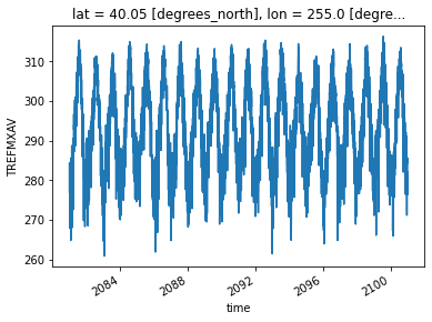
data visualization

ds["TREFMXAV"].plot()

[<matplotlib.lines.Line2D at 0x2b747263b2b0>]

Step 2: automated machine learning

train a model (emulator)

%%time
# assume that we want to split the data into training data and testing data
# let's use first 95% for training, and the remaining for testing
idx = df.shape[0]
train = df.iloc[:int(0.95*idx),:]
test = df.iloc[int(0.95*idx):,:]
(X_train, y_train) = (train[features], train[label].values)
(X_test, y_test) = (test[features], test[label].values)

# train the model
automl.fit(X_train=X_train, y_train=y_train,
           **automl_settings, verbose=-1)
print(automl.model.estimator)

LGBMRegressor(colsample_bytree=0.7463308378914483,
              learning_rate=0.1530612501227463, max_bin=1023,
              min_child_samples=2, n_estimators=60, num_leaves=49,
              reg_alpha=0.0009765625, reg_lambda=0.012698515198279536,
              verbose=-1)
CPU times: user 3min 20s, sys: 2.53 s, total: 3min 22s
Wall time: 15.2 s

apply and test the machine learning model

use automl.predict(X) to apply the model

# training data
print("model performance using training data:")
y_pred = automl.predict(X_train)
print("root mean square error:",
      mean_squared_error(y_true=y_train, y_pred=y_pred, squared=False))
print("r2:", r2_score(y_true=y_train, y_pred=y_pred),"\n")
import pandas as pd
d_train = {"time":train["time"],"y_train":y_train.reshape(-1),"y_pred":y_pred.reshape(-1)}
df_train = pd.DataFrame(d_train).set_index("time")

# testing data
print("model performance using testing data:")
y_pred = automl.predict(X_test)
print("root mean square error:",
      mean_squared_error(y_true=y_test, y_pred=y_pred, squared=False))
print("r2:", r2_score(y_true=y_test, y_pred=y_pred))
d_test = {"time":test["time"],"y_test":y_test.reshape(-1),"y_pred":y_pred.reshape(-1)}
df_test = pd.DataFrame(d_test).set_index("time")

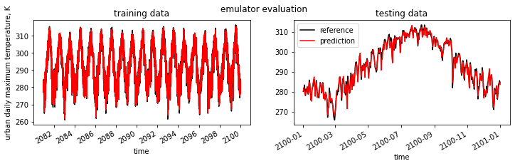
model performance using training data:
root mean square error: 1.0953179201882188
r2: 0.9908044117105271

model performance using testing data:
root mean square error: 1.6714483065300212
r2: 0.9799441548983633

visualization

fig, (ax1,ax2) = plt.subplots(1,2,figsize=(12,3))
fig.suptitle('emulator evaluation')
df_train["y_train"].plot(label="reference",c="k",ax=ax1)
df_train["y_pred"].plot(label="prediction",c="r",ax=ax1)
ax1.set_title("training data")
ax1.set_ylabel("urban daily maximum temperature, K")

df_test["y_test"].plot(label="reference",c="k",ax=ax2)
df_test["y_pred"].plot(label="prediction",c="r",ax=ax2)
ax2.set_title("testing data")
plt.legend()
plt.show()